1 Introduction
The aim of this document is to give a very broad overview of artificial intelligence or machine learning from the point of view of a commodity centric hedge fund. We will start off by looking at the two main branches of machine learning
- supervised learning
- unsupervised learning
A great way to view this landscape is through a series of examples. Traditionally these concepts are introduced on classic datasets such as
- Iris,
- MPG, and
- Housing Price.
Since we are a commodity trading house we will deviate from these examples and rather focus on datasets closer to what we deal with on a day to day basis. The overriding idea behind any machine learning algorithm is the need to generalise the results of the data given some set of input features. In this sense, even something very simple, like linear regression, can be used to generalise the information contained in a dataset.
In the first section, we introduce supervised learning and give an example of a regression and classification problem using commodity price and some fundamental data. This section also introduces some key concepts of machine learning:
- Splitting your data into training and testing sets
- Performing cross validation on your training sample
- Hyperparameter tuning
These methods are critical in creating models that perform well out of sample, i.e. on data that it has not seen during the training process. These techniques will be used for all models and examples shown. The second section introduces unsupervised learning with an example of how this can be used in a commodity setting to distinguish between two different regimes. In the third section, we show another use of machine learning algorithms that we find particularly interesting, feature importance.
We end this write-up with some general remarks on the use of machine learning and artificial intelligence on time series data. Throughour we include a number of interesting links to external articles that can be used to add to the content below.
2 Supervised Learning
2.1 General Idea
In supervised learning, we have a set of input features \(X\) and a collection of true values \(y\) associated with each of these features. Our goal is to find some function \(f\) such that
\[ f(X) = y + \epsilon \in \mathbb{R} \] where \(\epsilon\) is some (hopefully) small error term. There are two classes of supervised learning problems, regression and classification. Regression models are trained to give a real number as the output of \(f\). Classification models are used to determine the category associated with a collection of input features.
2.2 Calendar Spread Regression Example
Let us consider an example of supervised learning applied to the Chicago Corn ZZ calendar spreads. We define the value of the calendar spread as
\[ S_{Z_i, Z_{i+1}} := P_{Z_i} - P_{Z_{i+1}} \] where \(P_{Z_i}\) represents the price of the \(Z_i\) contract. As input features, we consider the front month price \(P_{Z_i}\) and stock-to-usage percentages as determined from the monthly WASDE publication. In this example we have WASDE data going back to July 1998. The spread data between two consecutive WASDE reports is connected to the data from the earlier report. The idea is then to take the WASDE data as a true representation of the underlying fundamentals and to use these fundamental inputs to model the value of the corn ZZ spread.
As a first step in the modeling of the data, it is always a good idea to visually inspect the data. Intuitively we expect to see a decreasing spread with increasing stock-to-usage. Fundamentally we also expect this effect to become smaller with increasing stock-to-usage where the spread approaches the fully carry value as the stock-to-usage approaches infinity. This behaviour is characteristic of exponential decay. The plot below confirms our intuition. The current values of the WASDE stock-to-usage and C ZZ spread is indicated by the vertical and horizontal lines respectively. The blue curve with shadow shows a loess fit to the underlying data.
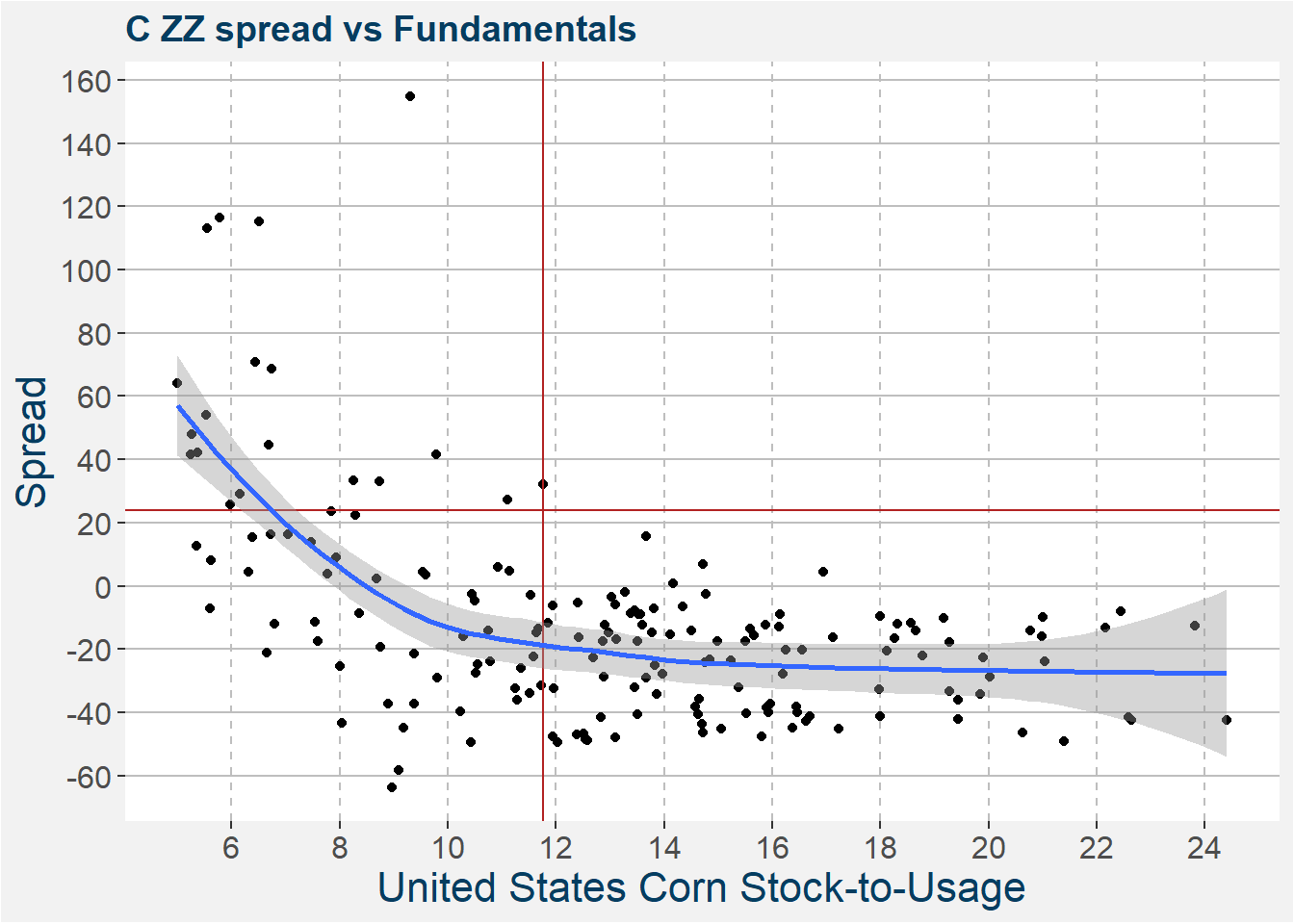
From above notice that the fit has decreasing slope and captures the general expected results. What is also clear from the above plot is that the relationship is not linear.
A fundamental idea in the machine learning literature is the concept of a training and testing set. To get a better idea of how a model will perform out of sample it is important to test your models on data that was not used in the construction of the model. A good rule of thumb is to use 20% of your dataset for out of sample testing. The above dataset consists of 199 data points. We pick 39 points at random and keep them for testing purposes. The remaining 160 data points are used in the training process.
In order to capture the general non-linear behaviour in the data, we use a kNN-algorithm. The algorithm is pretty intuitive, given an input value \(x\) for the United States Corn Stock-to-Usage, it looks at those \(k\) Nearest Neighbour datapoints in the training set which are closest to \(x\). The model then chooses the mean spread associated with each of those \(k\) data points as the output value.
An important step in training any machine learning algorithm is cross validation. Cross validation splits observations into two sets, one used for training and the other for testing. Each observation in the complete dataset belongs to one, and only one set. This is done to prevent leakage from one set into the other. If this is not done it would defeat the purpose of testing on unseen data. One of the more popular cross validation schemes is called k-fold cross validation. The figure below illustrates the k train/test splits carried out by a k-fold cross validation, where \(k=5\). The process goes as follows:
- The dataset is partitioned into \(k\) subsets
- For \(i = 1, \dots, k\)
- The machine learning algorithm is trained on all subsets excluding \(i\)
- The fitted machine learning algorithm is tested on \(i\)
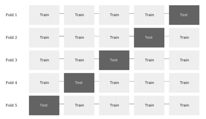
Five fold cross validation - (Image taken from Advances in Financial Machine Learing)
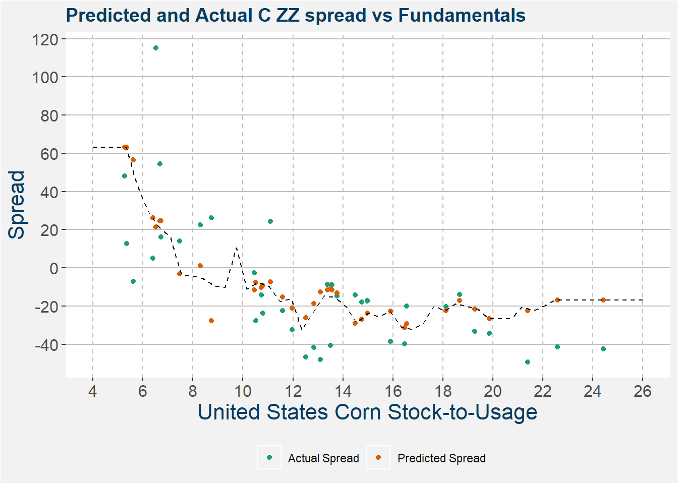
The plot below shows the model represented by the dashed black line. The actual and predicted spreads are indicated by the red and blue dots respectively. Notice that the model does a pretty decent job in describing the nonlinear relationship within the data. One big drawdown of this type of model is that it does not generalize well to test data outside of the range of the training data.
The interested reader can have a look at the links below for some more examples of research problems where we used regression models
The idea behind these three write-ups was the explore the links between global supply and demand and the outright price of the commodities. Once these models have been created we use them to test the feature sensitivity associated with individual input features. In this way, you can find possible critical points in the fundamentals which might cause significant price moves. These results are then combined with rigorous fundamental forecasting and stress testing to prod the balance sheets of the main producing and consuming nations. The stressed fundamentals are then passed to the models. If these stressed fundamentals coincide with significant price moves as predicted by the model it adds a layer of conviction to a trade. This type of quantamental approach plays a major part in how we will eventually size up a position.
2.3 Using classification to help determine bet sizing
This section will be a little bit more technical, but it illustrates an idea that is used within the Polar Star Quantitative Commodity Fund when sizing positions. Within the Polar Star Quantitative Commodity Fund, we have a strategy that takes systematic positions in calendar spreads. A calendar spread is a futures position where we take up opposing positions on the front and deferred sides of the futures curve of a single commodity. From the previous section, it should be clear that it is important to label your trading data correct when dealing with supervised learning. In the following, we introduce the idea of meta-labeling.
For a detailed discussion on how to label time series data for use in machine learning applications, the work of Marcos Lopez de Prado is invaluable. This is a must-read book for anybody interested in applying machine learning to time series data. In chapter 3 Marcos introduces the concept of meta-labeling.
The first step is in deciding the side of your bet, i.e. to take a long or short position. Below we suppose this has already been done either by some quantitative or discretionary method. What is left, is to decide the size of the bet, which includes the possibility of no bet at all. Below we simplify the problem to either taking the bet or not, i.e. we transform the problem to binary classification. The labeling is determined from looking at the return of the spread between successive rebalance periods. If the return is positive and above some predefined threshold it is labeled with a 1 (true), otherwise it is labeled with a 0 (false). This labeling defines the y or correct output of the classification function f we are trying to determine. For the input features X of these models we use a collection of lagged time series calculations which include
- autocorrelations,
- momentum,
- trend,
- mean reverting indicators as well as
- the side of the bet.
Our aim is then to fund the funciton \(f\) such that
\[ f(X) = y \in \left\{ 0, 1 \right\} \]
where the inpute features are
\[ X = \left(\begin{array}{ccccc} \text{autocorrelations}(t_1) & \text{momentum}(t_1) & \text{trend}(t_1) & \dots & \text{side}(t_1) \\ \vdots & \vdots & \vdots & \ddots & \vdots \\ \text{autocorrelations}(t_n) & \text{momentum}(t_n) & \text{trend}(t_n) & \dots & \text{side}(t_n) \end{array}\right) \]
The idea is that certain time series properties might have some predictive power in forecasting whether a bet will be profitable or not. Sticking with corn we consider the results of a simple Random Forest Classification model on corn calendar spreads using the scheme outlined above. Naturally, we have also used
- training and testing sets,
- k-fold cross validation, and
- hyperparameter tuning
in the construction of the classification model. Because we are dealing with time series data there are a couple of finer details and technicalities involved in the splitting between testing and training sets as well as the cross validation. These details amount to removing all lookahead bias and possible data leakage from out of sample data into the training data. For details on this, the book by Marcos Lopez de Prado serves as a great place to start.
The results of the model can be summarised in the confusion matrix below. The columns represent the true values, which in this case is a 1 if the position realised a profit and 0 if it realised a loss. The model predictions, of whether to take the bet or not, is shown on the rows.
| Actual Negative | Actual Positive | |
|---|---|---|
| Predict Negative | 1409 | 1236 |
| Predict Positive | 993 | 1751 |
The confusion matrix can also be visualised using the image below. Here the left and right halves of the box represents the actual positive and negative classes respectively. The abbreviations refer to
- TP: True Positive
- TN: True Negative
- FP: False Positive
- FN: False Negative
Here, true positives refer to the positive predictions that turned out to be true. A similar argument holds for the true negatives. The false positives refer to those entries marked positive but which should have been classified as negatives. The same argument holds for the false negatives.
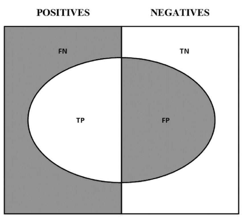
A visualisation of the confusion matrix - (Image taken from Advances in Financial Machine Learing)
From the confusion matrix below we can define a couple of useful quantities that are valuable in evaluating binary classifiers. Define Precision as the ratio between the TP are and the area in the ellipse. Define Recall as the ratio between the TP area and the area in the left rectangle. Accuracy is the ratio of the ellipse to the rectangle. A general rule of thumb is that decreasing the FP area comes at the cost of increasing the FN area. This is because higher precision typically means fewer calls, hence lower recall. There is also a combination of precision and recall that maximises the overall efficiency of a classifier, this is called the F1-score and is defined as the harmonic mean between precision and recall.
The table below shows the performance of the classifier according to the measures defined above. The columns “No Mask” and “With Meta-Labeling” show compare the results after adding the machine learning classifier to the original side of the bet. Notice the measured improvements in accuracy and precision. Adding the mask will result in greater profits and lower drawdowns. It also comes with the added benefit of reducing the turnover in your portfolio thereby reducing the overall trading costs.
| No Mask | With Meta-Labeling | |
|---|---|---|
| Accuracy | 0.554 | 0.586 |
| F1 | 0.713 | 0.611 |
| Precision | 0.554 | 0.638 |
| Recall | 1.000 | 0.586 |
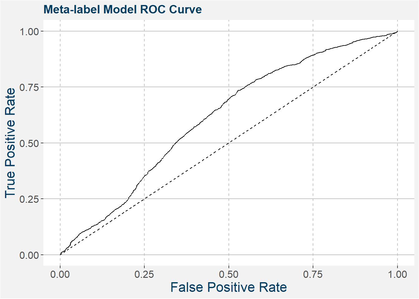
Another way to inspect the quality of these binary classification models is to use receiver operating characteristic (ROC) curves. These plots show the true positive rate (recall) as a function of false positive rate. The closer this graph gets to the top left corner of the graph the better classifier it is. For this reason, a measure that is often used to gauge the quality of a classifier is the area under the curve (AUC). The closer this number is to 1 to better classifier it is. A completely random classifier, basically a coin flip, yields the dashed line with slope 1 and AUC of 1/2. The hope is that our classifier will at least be better than a coin flip. The plot below shows the receiver operator curve of your meta-labeling model on the corn calendar spreads. We can see that it performs better than a random coin flip.
Some other interesting classification problems include:
- For a given front month price, will the curve be in backwardation or contango?
- Given the current rainfall data over the United States corn-producing area, should we expect a yield that is greater or less than the USDA?
- Given the global balance sheets for wheat, will the US vs Europe wheat trade yield a positive or negative roll?
Basically any question that can be framed so that it has a yes or no answer can be modeled using a classification algorithm.
3 Unsupervised Learning
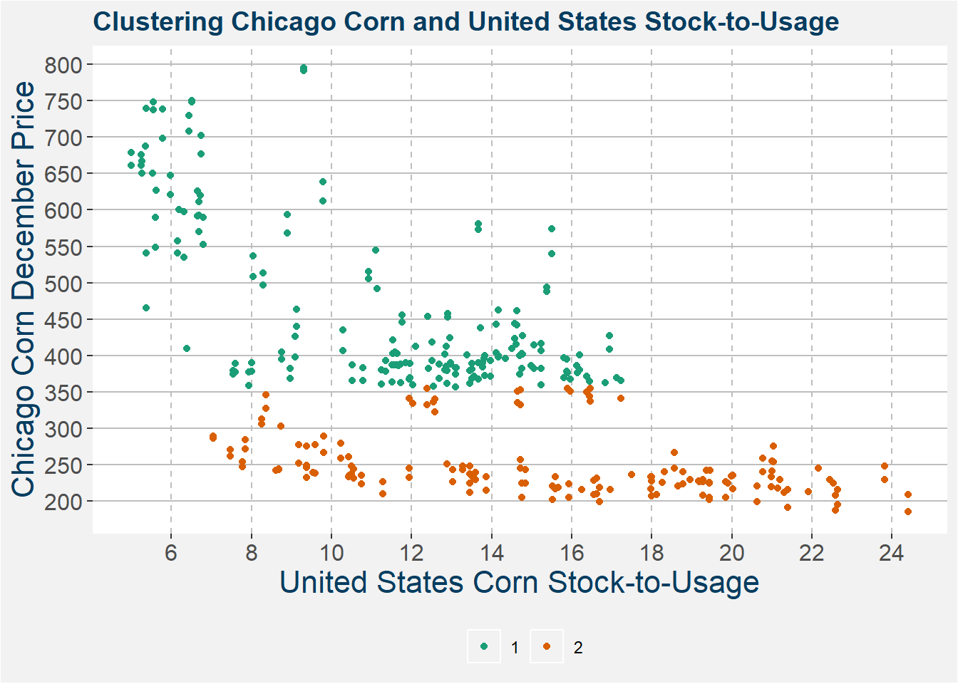
Unsupervised learning is different from supervised learning in that we do not give the model the correct of \(y\)-values. Instead, we ask the model to group the data into similar clumps. A standard model used to achieve this result is called k-means clustering. In the example below, we use the k-means clustering algorithm to group corn data into two groups. The results of this clustering are shown in the image below. The only input we gave the model was the split the data into two groups with the greatest difference.
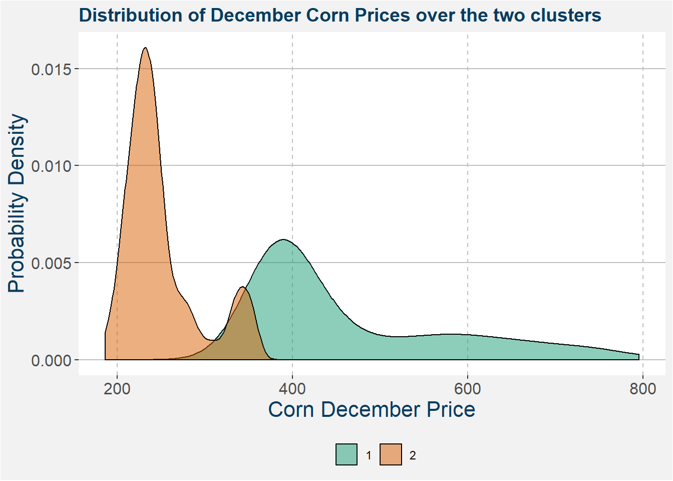
The eye the difference between the two clusters above seems more or less logical. In the plot below we show the distribution of December corn prices. Here the difference becomes even more clear and we can clearly see two distinct regimes.
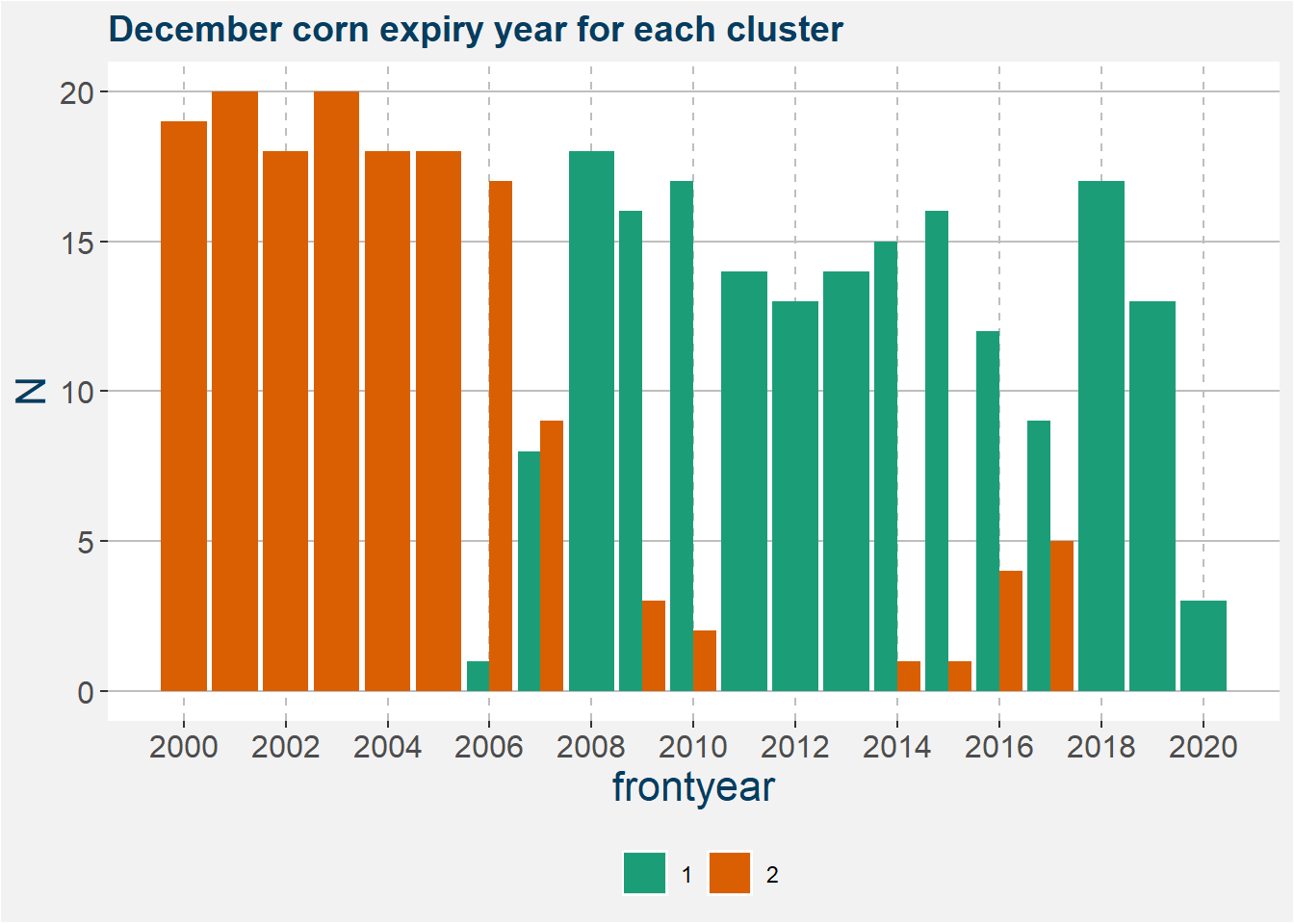
The plot below shows a barplot of the number of points for each of the expiry years. It is interesting to note the area where the cluster 2 merges into cluster 1. This gives a break in the data before and after 2008. This split is interesting because it coincides with the timeframe where the United States started to place an emphasis on ethanol production. This increase in the demand for corn fundamentally changed the corn market.
These types of clustering algorithms are usefull in determining structural breaks in markets. It is also useful in determining different volatility regimes. This is important in portfolio construction where larger positions will be built during regimes of low volatility in order to reach your target level of risk.
4 Feature Importance
This section comes directly from the Corn price vs Stock-to-Usage write-up.
We have created ensemble machine learning models that predict the corn price along the futures curve. These models take as inputs the stock-to-usage percentages of the top corn producing and consuming nations together with the dollar index and month prior average crude price as proxies for the US Dollar and energy respectively.
The ensemble models we create are all random forest regression models. We create a train and test split and perform hyperparameter tuning on the training set using 3 fold cross-validation. Within the training data, we perform oversampling to the less representative feature ranges. For more information on how to perform oversampling correctly, we refer the interested reader to this link. Ensemble models are a natural extension of the single variable deterministic models in that they are able to gain predictive quality from possible interactions between the different input features.
From the best models, we determine the variable importance of all the input features. The results are sumarised in the plot below. The greater the importance the larger the effect of that feature on the predicted values.
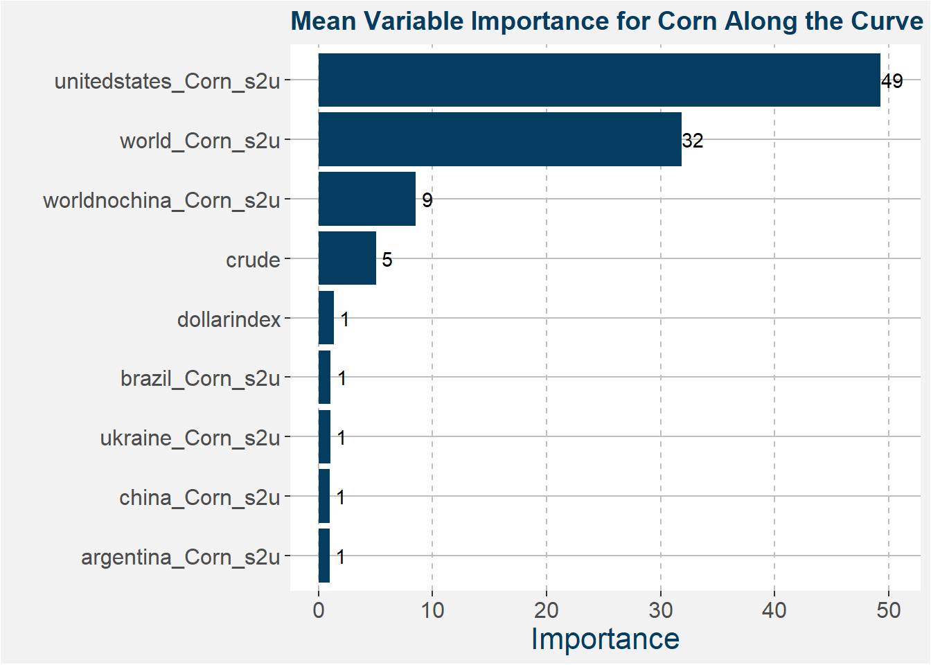
These results show that the main driving features in the United States corn market are the United States and world corn stock-to-usage numbers.
5 Remarks
Machine learning and artificial intelligence are buzzwords that many money managers have started throwing around. The truth is that these ideas have been available for a long time and have only recently received their place in the limelight because of the success that the tech industry has had with applications like image recognition and self-driving cars. It is also important to notice the differences between the classic uses of machine learning and what can be achieved in the realm of finance.
One key distinguishing feature is the form of your feature space. Classic machine learning is developed on the assumption that your features are drawn from independent and identically distributed random variables. In normal English, this means that the space from which your features are chosen remains more or less constant. In the language of time series analysis, this means that your features need to come from a stationary distribution, i.e. one that does not change over time. The vast majority of financial time series data is not stationary. Feeding this into any off-the-shelf machine learning algorithm will result in models that perform poorly out of sample.
The nature of time series and the issues related to data leakage can cause havoc on machine learning algorithms’ performance on out of sample data. These and other issues are addressed in The 10 Reasons Most Machine Learning Funds Fail by Lopez de Prado.